Cosmology Models
Flat Space: k = 0 with cosmological constant
Assuming that we are dealing with a spatially flat universe with zero pressure, the Friedmann equation becomes the following:
|
|
|
We look at the solution of this differential equation when
|
(30.2) |
|
|
For convenience in solving the differential equation we now change the dependent variable as follows
|
|
|
Take the first-order derivative of this equation on both sides:
|
(30.4) |
|
|
Using the Friedmann evolution equation in this result gives the following expression.
|
(30.5) |
|
|
Using the definition (30.3) this equation can be rewritten in the manner:
|
(30.6) |
|
|
Since we are considering a growing universe, we take the positive root of this expression
|
|
|
Our initial conditions are as follows:
|
|
|
Using these conditions one integrates (30.7) as follows:
|
(30.9) |
|
|
This gives
|
(30.10) |
|
|
Substituting to get the scale factor back in this equation gives the evolution when the cosmological constant is positive.
|
(30.11) |
|
|
Consider the case where
|
(30.12) |
|
|
This time define a new dependent variable this way:
|
(30.13) |
|
|
Using the same integration technique as before in the positive case we get the following solution in the negative cosmological constant case.
(30.14)
The third possible case is where
|
(30.15) |
|
|
The Friedmann evolution becomes
|
(30.16) |
|
|
In differential form this becomes:
|
(30.17) |
|
|
The initial conditions (30.8) then imply that
|
(30.18) |
|
|
Solving for we get
|
(30.19) |
|
|
This evolution model is famous in that it was studied both by Einstein and the Dutch physicist de Sitter. It is called the Einstein-de Sitter model for the matter-dominated universe.

For information on Willem de Sitter go to the following page:
http://www.phys-astro.sonoma.edu/BruceMedalists/deSitter/
It is sometimes useful to calculate the
second-order derivative of the scale factor using the following combination of
terms called the deceleration parameter, .
|
(30.20) |
|
|
Equivalently, this is also written
|
(30.21) |
|
|
In the Einstein- de Sitter case
|
(30.22) |
|
|
Qualitative Behaviour: with
Constant
We can get information about the solutions
of the case without solving the equations. To do
this we observe how the function of R that is on the right hand side of the
Friedmann equation (30.1)
behaves.
|
(30.23) |
|
|
Note the following about this equation.
|
(30.24) |
|
|
|
(30.25) |
|
|
Furthermore in the case where ,
we have a local maximum occurring at
|
(30.26) |
|
|
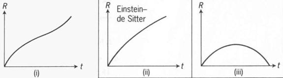
The graphs for are shown below.
Curved 3-D Space: with
Constant
The Friedmann equation in the case where the cosmological constant is zero is
|
(30.27) |
|
|
The case where
The Friedmann equation is
|
|
|
|
(30.29) |
|
|
Upon differentiation this gives
|
(30.30) |
|
|
The Friedmann equation (30.28) can then be reworked to give
(30.31)
For an expanding universe we take the positive square root and put the initial conditions into the integral as follows:
|
(30.32) |
|
|
This integrates to the following:
|
(30.33) |
|
|
Putting back the scale factor R(t) we get the following evolution equation:
|
(30.34) |
|
|
This is a transcendental equation but it is not hard to figure out how this evolution equation describes this type of universe.
The case where
Using a similar solving technique we can get the solution of the Friedman equation in this case
|
(30.35) |
|
|
The solution also is a transcendental type of equation similar in form to the positive curvature case
|
(30.36) |
|
|
Qualitative Behaviour: with
Constant
|
(30.37) |
|
|
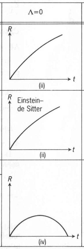
The case is the same as before: the Einstein-de Sitter
solution.
|
(30.38) |
|
|
|
(30.39) |
|
|
The graphs for are respectively shown below.
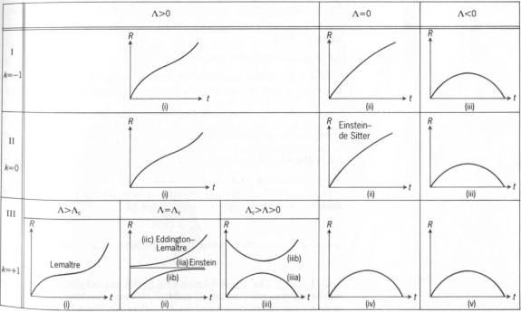
The graphs of all possible solutions of the Friedmann equation
|
(30.40) |
|
|
are shown in the diagrams below.